Classification is a type of Supervised Machine Learning method of classifying new input data after the model has learnt to classify the training data provided to it. It identifies the set of categories a new observation belongs to on the basis of a set of training data containing observations (or instances) whose category is known. The observations (or instances) are termed as Explanatory Variables/Features/Independent Variables and the categories to be predicted are known as Outcomes/Classes which are considered to be the possible values of the Target/Dependent Variables. Classification can be considered as an example of pattern recognition (which assigns some sort of output value to a given input value).
A machine learning algorithm that implements classification is known as a “Classifier”. In mathematical terms, it is a function (f) that maps input data (X) to a category/discrete output variable (Y). Examples of application of Classification in the real world may include email spam/ham filter, speech recognition, diabetes prediction, handwriting recognition, biometric identification, document classification etc.
A machine learning classification problem can be thought of two separate problems – Binary Classification and Multiclass Classification. In a binary classification problem, only two classes/outcomes are involved whereas in a multiclass classification problem, the new input data can be assigned to multiple classes/outcomes. A simple example of a binary classification can be classification of whether an incoming email is a spam or a ham (not spam). The 2 classes here are “spam” and “ham”. Let’s consider you want to predict whether the weather of the upcoming days will be sunny/windy/rainy. The classes here are “sunny”, “windy” and “rainy”. This is a multiclass classification problem and such kind of classification requires combined use of multiple binary classifiers.
A classifier can also be categorized as a Linear Classifier or a Non-Linear Classifier. A classifier is “linear” when its decision boundary on the feature space is a linear function, that is, the data are linearly separable – the points belonging to class 1 can be separated from the points belonging to class 2 by a hyperplane. If the decision boundary is a non-linear function, that is, the data are non-linearly separable, then the classifier is a “non-linear classifier”. The non-linear problem, in most cases, are solved by applying a transform to the data points to feature space with a hope that in feature space the data points will be linearly separable. The higher the dimension of the feature space, the greater the number of data points that are linearly separable in that space. Therefore, one would ideally want the feature space to be as high-dimensional as possible, but it would lead to increased computation. In such cases, the algorithms can be formulated in such a way that the only operation that they perform on the data points is a scalar product between the data points. We can evaluate this scalar product in both lower-dimensional and higher-dimensional feature space.
The various types of Classification techniques are:
Linear Classification:
- Logistic Regression
- Support Vector Machine (SVM)
Non-Linear Classification:
- K-Nearest Neighbor (K-NN)
- Kernel SVM
- Naïve Bayes Classification
- Decision Tree Classification
- Random Forest Classification
LOGISTIC REGRESSION
Logistic Regression is a Supervised Machine Learning classification technique which is used to explain the relationship between one dependent/target variable (categorical) and one or more nominal, ordinal, interval or ratio-level independent/explanatory variables.
Based on the possible outcomes, Logistic Regression can be of 3 types:
Binary Logistic Regression: Deals with 2 possible binary outcomes (Yes/No, 1/0, True/False). For example, detecting whether an email is a spam email or not.
Multinomial Logistic Regression: Deals with 3 or more, order-less, categorical outcomes (Red/Green/Blue, Sunny/Windy/Rainy, Veg/Non-Veg/Vegan etc.).
Ordinal Logistic Regression: Deals with 3 or more, ordered, categorical outcomes (Customer Rating of an eShop from 1 to 10).
Though the name “Logistic Regression” consists of the term “Regression”, it is not a Regression technique. Rather, it is a classification technique and is quite popular among the machine learning engineers to address Classification problems.
Logistic Regression Intuition
Though Logistic Regression is a linear method, the predictions are transformed using the mathematical function known as “Logistic Function” (also known as the “Sigmoid Function”) which is at the core of Logistic Regression. The Logistic/Sigmoid Function is an S-shaped curve that can take any real-valued number and map it between the values 0 and 1 (but not exactly at the limits).
We already know, y = b0 + b1x ………………………. eq(1)
Sigmoid Function (p) = 1/(1+e-y) ………………………. eq(2)
=> p + pe-y = 1
=> pe-y = (1-p)
=> e-y=(1-p)/p
=>1/ey = (1-p)/p
=> y = ln(p/(1-p))
Hence, ln(p/(1-p)) = b0 + b1x ………………………. eq(3)
=> p/(1-p)=e^(b0 + b1x) ……………………………….. eq(4)
where, p = probability
e = base of natural logarithms/Euler’s number
y = predicted output
x = Input values
b0= Bias or Intercept term
b1= Co-efficient for the single input value x
p/(1-p) = Odds of the default class or Ratio of event probability/Probability of not the event
From the above equation eq(3), we can see that the output calculation on the right is linear (like linear regression) and the input on the left is a log of the probability of the default first class.
Thus, we can say that logistic Regression models the probability of the default first class. For example, if we are modelling spam email or ham email from its content, then the first class could be “spam email” and the logistic regression model could be written as the probability of spam email given an email’s content. Mathematically, the probability can be given as:
P(email=spam|content)
In other words, we are modelling the probability that an input (X) belongs to the default class (Y=1)
P(X)=P(Y=1|X)
Let’s now consider a dataset (Car_Purchase) which provides information on whether the employees of a firm have purchased car or not based on other independent variables like age and estimated salary. You can find the data from here. Let’s see the Python implementation:
# Logistic Regression

# Import the required libraries and the collected dataset
import numpy as np
import pandas as pd
import matplotlib.pyplot as plotter
collectedDataset=pd.read_csv('Car_Purchase.csv')
X=collectedDataset.iloc[:,[2,3]].values
Y=collectedDataset.iloc[:,4].values

# Split the Dataset into the Training Set and Test Set with test size of 0.2
from sklearn.model_selection import train_test_split
X_train,X_test,Y_train,Y_test=train_test_split(X,Y,test_size=0.2,random_state=0)

# Perform Featue Scaling on the data points
from sklearn.preprocessing import StandardScaler
standardScaler_X=StandardScaler()
X_train=standardScaler_X.fit_transform(X_train)
X_test=standardScaler_X.transform(X_test)

# Fit the Logistic Regression Model to the Training Set
from sklearn.linear_model import LogisticRegression
logisticRegressionClassifier=LogisticRegression(random_state=0)
logisticRegressionClassifier.fit(X_train,Y_train)

# Predict the Test Set Results bqsed on the model
Y_predict=logisticRegressionClassifier.predict(X_test)

# Create the Confusion Matrix
from sklearn.metrics import confusion_matrix
cm=confusion_matrix(Y_test,Y_predict)

# Visualize the Training Set Results
from matplotlib.colors import ListedColormap
X_set, Y_set = X_train, Y_train
X1, X2 = np.meshgrid(np.arange(start = X_set[:, 0].min() - 1, stop = X_set[:, 0].max() + 1, step = 0.01),
                     np.arange(start = X_set[:, 1].min() - 1, stop = X_set[:, 1].max() + 1, step = 0.01))
plotter.contourf(X1, X2, logisticRegressionClassifier.predict(np.array([X1.ravel(), X2.ravel()]).T).reshape(X1.shape),
             alpha = 0.75, cmap = ListedColormap(('red', 'green')))
plotter.xlim(X1.min(), X1.max())
plotter.ylim(X2.min(), X2.max())
for i, j in enumerate(np.unique(Y_set)):
    plotter.scatter(X_set[Y_set == j, 0], X_set[Y_set == j, 1],
                c = ListedColormap(('red', 'green'))(i), label = j)
plotter.title('Logistic Regression (Training set)')
plotter.xlabel('Age')
plotter.ylabel('Estimated Salary')
plotter.legend()
plotter.show()

# Visualize the Test Set Results
from matplotlib.colors import ListedColormap
X_set, Y_set = X_test, Y_test
X1, X2 = np.meshgrid(np.arange(start = X_set[:, 0].min() - 1, stop = X_set[:, 0].max() + 1, step = 0.01),
                     np.arange(start = X_set[:, 1].min() - 1, stop = X_set[:, 1].max() + 1, step = 0.01))
plotter.contourf(X1, X2, logisticRegressionClassifier.predict(np.array([X1.ravel(), X2.ravel()]).T).reshape(X1.shape),
             alpha = 0.75, cmap = ListedColormap(('red', 'green')))
plotter.xlim(X1.min(), X1.max())
plotter.ylim(X2.min(), X2.max())
for i, j in enumerate(np.unique(Y_set)):
    plotter.scatter(X_set[Y_set == j, 0], X_set[Y_set == j, 1],
                c = ListedColormap(('red', 'green'))(i), label = j)
plotter.title('Logistic Regression (Test set)')
plotter.xlabel('Age')
plotter.ylabel('Estimated Salary')
plotter.legend()
plotter.show()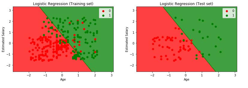
K-NN (K-NEAREST NEIGHBOR) ALGORITHM
K-Nearest Neighbor is a Supervised Machine Learning Classification technique (sometimes it is also used to solve Regression problems) where the input data consists of the k-closest training examples (‘k’ is typically a small positive integer), which are vectors in the multidimensional feature space and the output is a class membership/category. The training data classifies co-ordinates into groups identified by an attribute. A data point is classified by a plurality vote of its neighbors with the data point being assigned to the class/category which is most common among its k-nearest neighbors.
The ‘k’ is a user-defined constant. An unlabeled new test data point/vector is classified by assigning the label which is most frequent among the k-training examples nearest to the test data point. If k=1, then the data is simply assigned to the class/category of that single nearest neighbor
A common distance metric which is used to measure the distances in K-Nearest Neighbor Algorithm is the Euclidean Distance which is a straight line distance between two points in Euclidean space. Other popular distance metrics which can also be used are – Hamming, Manhattan/City Block, Tanimoto, Jaccard, Mahalanobis, Cosine and Minkowski Distance. Here, we will be using Euclidean Distance.
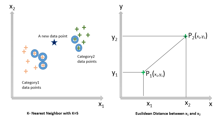
The Euclidean Distance between the points P1 and P2 is given by the formula:

KNN Steps
Step1: Load the data
Step2: Choose the number (K) of neighbors and initialize the value of k (In the above figure, k=5)
Step3: Take the k(=5) nearest neighbors of the new data point according to the Euclidean distance explained above
Step4: Among these K number of neighbors, count the number of data points in each category
Step5: Assign the new data point to the class/category where the most number of neighbors are present
Step6: Model is Ready
Let’s now consider the same dataset (Car_Purchase) which we have used for logistic regression previously. The python code implementation is below:
#KNN (K-Nearest Neighbors) Classification

# Import the required libraries and the collected dataset
import numpy as np
import pandas as pd
import matplotlib.pyplot as plotter
collectedDataset = pd.read_csv('Car_Purchase.csv')
X = collectedDataset.iloc[:, [2, 3]].values
Y = collectedDataset.iloc[:, 4].values

# Split the dataset into the Training set and Test set
from sklearn.model_selection import train_test_split
X_train, X_test, Y_train, Y_test = train_test_split(X, Y, test_size = 0.25, random_state = 0)

# Feature Scale
from sklearn.preprocessing import StandardScaler
standardScaler = StandardScaler()
X_train = standardScaler.fit_transform(X_train)
X_test = standardScaler.transform(X_test)

# Fit the KNN classifier to the Training set
from sklearn.neighbors import KNeighborsClassifier
classifier=KNeighborsClassifier(n_neighbors=5,metric='minkowski',p=2)
classifier.fit(X_train,Y_train)

# Predict the Test set results
Y_pred = classifier.predict(X_test)

# Make the Confusion Matrix
from sklearn.metrics import confusion_matrix
cm = confusion_matrix(Y_test, Y_pred)

# Visualize the Training set results
from matplotlib.colors import ListedColormap
X_set, Y_set = X_train, Y_train
X1, X2 = np.meshgrid(np.arange(start = X_set[:, 0].min() - 1, stop = X_set[:, 0].max() + 1, step = 0.01),
                     np.arange(start = X_set[:, 1].min() - 1, stop = X_set[:, 1].max() + 1, step = 0.01))
plotter.contourf(X1, X2, classifier.predict(np.array([X1.ravel(), X2.ravel()]).T).reshape(X1.shape),
             alpha = 0.75, cmap = ListedColormap(('red', 'green')))
plotter.xlim(X1.min(), X1.max())
plotter.ylim(X2.min(), X2.max())
for i, j in enumerate(np.unique(Y_set)):
    plotter.scatter(X_set[Y_set == j, 0], X_set[Y_set == j, 1],
                c = ListedColormap(('red', 'green'))(i), label = j)
plotter.title('K-NN (Training set)')
plotter.xlabel('Age')
plotter.ylabel('Estimated Salary')
plotter.legend()
plotter.show()

# Visualize the Test set results
from matplotlib.colors import ListedColormap
X_set, Y_set = X_test, Y_test
X1, X2 = np.meshgrid(np.arange(start = X_set[:, 0].min() - 1, stop = X_set[:, 0].max() + 1, step = 0.01),
                     np.arange(start = X_set[:, 1].min() - 1, stop = X_set[:, 1].max() + 1, step = 0.01))
plotter.contourf(X1, X2, classifier.predict(np.array([X1.ravel(), X2.ravel()]).T).reshape(X1.shape),
             alpha = 0.75, cmap = ListedColormap(('red', 'green')))
plotter.xlim(X1.min(), X1.max())
plotter.ylim(X2.min(), X2.max())
for i, j in enumerate(np.unique(Y_set)):
    plotter.scatter(X_set[Y_set == j, 0], X_set[Y_set == j, 1],
                c = ListedColormap(('red', 'green'))(i), label = j)
plotter.title('K-NN (Test set)')
plotter.xlabel('Age')
plotter.ylabel('Estimated Salary')
plotter.legend()
plotter.show()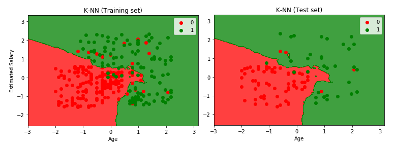
SUPPORT VECTOR MACHINE (SVM)
Support Vector Machine (popularly known as SVM) is a Supervised Machine Learning Classification technique which can be used to perform binary classification analysis on the collected data. The concept behind SVM is that when it is provided with labeled training data, it is able to output an optimal hyperplane which will categorize the new test data points. A hyperplane is an imaginary line which divides a plane in two parts and each binary class represents each side.
Consider the below diagrams:
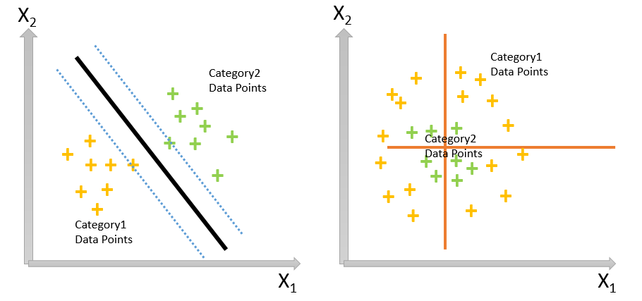
Consider Figure1 – if you are given a plot of two label classes/categories distributed in the diagram, then you can easily decide a separating line/decision boundary between the two categories and the related support vectors. Now, for a new test data point, if it resides on the left side of the line, it will be classified to Category1 and if on the right side, it will be classified to Category2. What will happen if the data points of the two categories are distributed like Figure2? We will not be able to draw a clear separating line between the categories and here comes the concept of hyperplane in the multidimensional space to find the best decision boundary. The hyperplane will maximize the margin between the two categories, with the help of the support vectors, in the N-dimensional space and we will be able to categorize a new test data point on the basis of this hyperplane.
Let’s consider the same dataset (Car_Purchase) which we have used for logistic regression and KNN. The python code implementation for SVM is given below:
# Support Vector Machine (SVM)

# Import the required libraries and the collected dataset
import pandas as pd
import numpy as np
import matplotlib.pyplot as plotter
collectedDataset = pd.read_csv('Car_Purchase.csv')
X = collectedDataset.iloc[:, [2, 3]].values
Y = collectedDataset.iloc[:, 4].values

# Split the dataset into the Training set and Test set
from sklearn.model_selection import train_test_split
X_train, X_test, Y_train, Y_test = train_test_split(X, Y, test_size = 0.25, random_state = 0)

# Feature Scale
from sklearn.preprocessing import StandardScaler
standardScaler = StandardScaler()
X_train = standardScaler.fit_transform(X_train)
X_test = standardScaler.transform(X_test)

# Fit the SVM to the Training set
from sklearn.svm import SVC
suuportVectorClassifier=SVC(kernel='linear',random_state=0)
suuportVectorClassifier.fit(X_train,Y_train)

# Predict the Test set results
Y_predict = suuportVectorClassifier.predict(X_test)

# Make the Confusion Matrix
from sklearn.metrics import confusion_matrix
confusionMatrix = confusion_matrix(Y_test, Y_predict)

# Visualize the Training set results
from matplotlib.colors import ListedColormap
X_set, Y_set = X_train, Y_train
X1, X2 = np.meshgrid(np.arange(start = X_set[:, 0].min() - 1, stop = X_set[:, 0].max() + 1, step = 0.01),
                     np.arange(start = X_set[:, 1].min() - 1, stop = X_set[:, 1].max() + 1, step = 0.01))
plotter.contourf(X1, X2, suuportVectorClassifier.predict(np.array([X1.ravel(), X2.ravel()]).T).reshape(X1.shape),
             alpha = 0.75, cmap = ListedColormap(('red', 'green')))
plotter.xlim(X1.min(), X1.max())
plotter.ylim(X2.min(), X2.max())
for i, j in enumerate(np.unique(Y_set)):
    plotter.scatter(X_set[Y_set == j, 0], X_set[Y_set == j, 1],
                c = ListedColormap(('red', 'green'))(i), label = j)
plotter.title('Support Vector Machine (Training set)')
plotter.xlabel('Age')
plotter.ylabel('Estimated Salary')
plotter.legend()
plotter.show()

# Visualize the Test set results
from matplotlib.colors import ListedColormap
X_set, Y_set = X_test, Y_test
X1, X2 = np.meshgrid(np.arange(start = X_set[:, 0].min() - 1, stop = X_set[:, 0].max() + 1, step = 0.01),
                     np.arange(start = X_set[:, 1].min() - 1, stop = X_set[:, 1].max() + 1, step = 0.01))
plotter.contourf(X1, X2, suuportVectorClassifier.predict(np.array([X1.ravel(), X2.ravel()]).T).reshape(X1.shape),
             alpha = 0.75, cmap = ListedColormap(('red', 'green')))
plotter.xlim(X1.min(), X1.max())
plotter.ylim(X2.min(), X2.max())
for i, j in enumerate(np.unique(Y_set)):
    plotter.scatter(X_set[Y_set == j, 0], X_set[Y_set == j, 1],
                c = ListedColormap(('red', 'green'))(i), label = j)
plotter.title('Support Vector Machine (Test set)')
plotter.xlabel('Age')
plotter.ylabel('Estimated Salary')
plotter.legend()
plotter.show()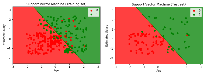
KERNEL SVM
“Kernels” are mathematical functions which take data (sequence data, graphs, text, images, vectors) as input and transform the data into the required form. SVM algorithms can use different Kernel functions like Gaussian Kernel, Gaussian RBF (Radial Basis Function) Kernel, Laplace RBF Kernel, Hyperbolic Tangent Kernel, Sigmoid Kernel, Linear Kernel, Non-linear Kernel, Polynomial Kernel, ANOVA Radial Basis Kernel, Scalar Product Kernel, Squared Distance Kernel, Sine Squared Kernel, Chi-Squared Kernel, Periodic Kernel, Rational Quadratic Kernel, Matern Kernel etc. Sometimes, in normal SVM, mapping the data points to a higher dimensional space can be highly compute-intensive. The kernel functions return the inner product between two data points in a feature space which makes Kernel SVMs less compute-intensive in higher dimensional space.
In machine learning, the term “kernel” is usually used to refer to the “kernel trick” which is a technique of using a linear classifier to solve a non-linear problem by transforming linearly inseparable data to linearly separable. The kernel functions can be applied to each data point to map the original non-linear observations into a higher-dimensional space in which the data points become separable.
Kernel SVM Intuition
The mathematical Kernel function is defined as:
K(x, y) = <f(x), f(y)>
where, K is the kernel function
x, y are n dimensional inputs
f is a map from n-dimension to m-dimension space
<x,y> denotes the dot product
Usually m is much larger than n
Let’s now take the same dataset (Car_Purchase) and see the implementation of Kernel SVM using python:
# Kernel Support Vector Machine (SVM)

# Import the required libraries and the collected dataset
import numpy as np
import matplotlib.pyplot as plotter
import pandas as pd
collectedDataset = pd.read_csv('Car_Purchase.csv')
X = collectedDataset.iloc[:, [2, 3]].values
Y = collectedDataset.iloc[:, 4].values

# Split the dataset into the Training set and Test set
from sklearn.model_selection import train_test_split
X_train, X_test, Y_train, Y_test = train_test_split(X, Y, test_size = 0.25, random_state = 0)

# Feature Scale
from sklearn.preprocessing import StandardScaler
standardScaler = StandardScaler()
X_train = standardScaler.fit_transform(X_train)
X_test = standardScaler.transform(X_test)

# Fit the Kernel SVM to the Training set
from sklearn.svm import SVC
kernelSVMClassifier=SVC(kernel='rbf',random_state=0)
kernelSVMClassifier.fit(X_train,Y_train)

# Predict the Test set results
Y_predict = kernelSVMClassifier.predict(X_test)

# Make the Confusion Matrix
from sklearn.metrics import confusion_matrix
confusionMatrix = confusion_matrix(Y_test, Y_predict)

# Visualize the Training set results
from matplotlib.colors import ListedColormap
X_set, Y_set = X_train, Y_train
X1, X2 = np.meshgrid(np.arange(start = X_set[:, 0].min() - 1, stop = X_set[:, 0].max() + 1, step = 0.01),
                     np.arange(start = X_set[:, 1].min() - 1, stop = X_set[:, 1].max() + 1, step = 0.01))
plotter.contourf(X1, X2, kernelSVMClassifier.predict(np.array([X1.ravel(), X2.ravel()]).T).reshape(X1.shape),
             alpha = 0.75, cmap = ListedColormap(('red', 'green')))
plotter.xlim(X1.min(), X1.max())
plotter.ylim(X2.min(), X2.max())
for i, j in enumerate(np.unique(Y_set)):
    plotter.scatter(X_set[Y_set == j, 0], X_set[Y_set == j, 1],
                c = ListedColormap(('red', 'green'))(i), label = j)
plotter.title('Kernel SVM Classification (Training set)')
plotter.xlabel('Age')
plotter.ylabel('Estimated Salary')
plotter.legend()
plotter.show()

# Visualize the Test set results
from matplotlib.colors import ListedColormap
X_set, Y_set = X_test, Y_test
X1, X2 = np.meshgrid(np.arange(start = X_set[:, 0].min() - 1, stop = X_set[:, 0].max() + 1, step = 0.01),
                     np.arange(start = X_set[:, 1].min() - 1, stop = X_set[:, 1].max() + 1, step = 0.01))
plotter.contourf(X1, X2, kernelSVMClassifier.predict(np.array([X1.ravel(), X2.ravel()]).T).reshape(X1.shape),
             alpha = 0.75, cmap = ListedColormap(('red', 'green')))
plotter.xlim(X1.min(), X1.max())
plotter.ylim(X2.min(), X2.max())
for i, j in enumerate(np.unique(Y_set)):
    plotter.scatter(X_set[Y_set == j, 0], X_set[Y_set == j, 1],
                c = ListedColormap(('red', 'green'))(i), label = j)
plotter.title('Kernel SVM Classification (Test set)')
plotter.xlabel('Age')
plotter.ylabel('Estimated Salary')
plotter.legend()
plotter.show()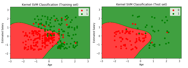
NAÏVE BAYES CLASSIFICATION
Naïve Bayes Classification is a Supervised Machine Learning Classification technique which is based on the Bayes’ Theorem with the assumption that the presence of a particular feature in a class is unrelated to the presence of any other feature. Due to this independence assumption, the Bayes’ theorem is called “Naive”. The independent variables might not always be completely independent from each other e.g. the features “Salary” and “Age” can have a correlation between each other. Consider, an employee having features of “Salary”, ”Age” and “Years of Experience”. Even if these features depend on each other or upon the existence of the other features, all of these properties independently contribute to the probability that this employee might join the company and that is the reason why the algorithm is known as “Naive”.
The Naïve Bayes Classifiers can be of different types:
1) Multinomial Naïve Bayes (used for discrete counts)
2) Bernoulli Naïve Bayes (binomial model which can be used if the features are binary (i.e. zeros and ones))
3) Gaussian Naïve Bayes (assumes that features follow a normal distribution.)
Now, let’s now try to understand how the basic Bayes Theorem works.
The Bayes’ Theorem is given by the below formula:
P(A | B) = (P(B | A)*P(A) )/ P(B)
where, P (A | B) is the Posterior Probability of class A (target/dependent variable) given predictor B (feature/attribute/independent variable/explanatory variables)
P(A) is the Prior Probability of class A
P(B | A) is the Likelihood probability of predictor B, given class A
P(B) is the Prior Probability of Predictor B (Marginal Likelihood – It is the likelihood that a randomly picked data will exhibit features similar to the datapoint that we are going to add)
Using the Bayes’ Theorem, we can find the probability of output A happening, given that the feature B has occurred. Here, B is the evidence and A is the hypothesis. The assumption made here is that the predictors/ features are independent which means that the presence of one particular feature does not affect the other features.
Let us consider the below dataset of a test execution getting passed or failed:
| Execution Time (in seconds) | Execution Type | Testing Type | Jenkins Used | Execution Result | |
| 0 | 20-40 | Web | System Test | Yes | Pass |
| 1 | 20-40 | Web | Integration Test | Yes | Pass |
| 2 | 10-20 | Web | Integration Test | Yes | Pass |
| 3 | 0-10 | Mobile | End To End Test | No | Fail |
| 4 | 10-20 | Web | End To End Test | Yes | Fail |
| 5 | 10-20 | Mobile | Integration Test | No | Pass |
| 6 | 60-120 | Mobile | System Test | No | Fail |
| 7 | 0-10 | Web | Integration Test | Yes | Pass |
| 8 | 20-40 | Mobile | System Test | Yes | Fail |
| 9 | 20-40 | Mobile | System Test | No | Fail |
| 10 | 20-40 | Mobile | IntegrationTest | Yes | Fail |
Here, we classify whether the test execution will get “Passed” or “Failed”, given the features of the test execution. The columns represent the features and the rows represent the individual entries. Consider the first row where we can observe that the test is getting “Passed” if the time taken for execution is between 20 to 40 seconds, the execution type is “Web”, the testing type is “System Test” and “Jenkins” executors have been used for execution. We have made 2 assumptions here:
1) The predictors are independent, that is, if the Test Execution type is “Web”, it does not necessarily mean that “Jenkins” executors have been used for its testing or the testing type is “System testing” only.
2) All the predictors have an equal effect on the outcome on whether the test is passed or failed.
According to this example, the Bayes’ Theorem can be rewritten as:
P(y | X) = (P(X | y)*P(y) )/ P(X)
where, y = dependent class or output variable (passed or failed)
X = parameters/features (Execution Time, Execution Type, Testing Type, Jenkins used)
Now, X can be given as:
X = (x1, x2,x3, ………………. , xn)
where, x1, x2, x3, ………… xn = Mapped to the parameters/features (Execution Time, Execution Type, Testing Type, Jenkins used)
By substituting for X and expanding using the chain rule, we get:
P(y | x1, …., xn) = (P(x1 | y)* P(x2 | y)* ……. P(xn | y) *P(y) )/ (P(x1)* P(x2)*…. P(xn))
Now, we can obtain the values for each by looking at the dataset and substitute them into the equation. For all entries in the dataset, the denominator does not change and remains static.
In this case, the class/ target/ output variable y has only two outcomes – “Passed” and “Failed”. There could also be cases where the classification could be multivariate, that is, multiple (n) number of categories/classes.
Let us now see the Python implementation of Gaussian Naïve Bayes Classifier using our previously used Car_Purchase dataset.
# Naive Bayes Classification

# Importing the required libraries and the collected Dataset
import numpy as np
import matplotlib.pyplot as plt
import pandas as pd
collectedDataset = pd.read_csv('Car_Purchase.csv')
X = collectedDataset.iloc[:, [2, 3]].values
Y = collectedDataset.iloc[:, 4].values

# Split the dataset into the Training set and Test set
from sklearn.model_selection import train_test_split
X_train, X_test, Y_train, Y_test = train_test_split(X, Y, test_size = 0.25, random_state = 0)

# Feature Scale
from sklearn.preprocessing import StandardScaler
standardScaler = StandardScaler()
X_train = standardScaler.fit_transform(X_train)
X_test = standardScaler.transform(X_test)

# Fit Gaussian Naive Bayes Classifier to the Training set
from sklearn.naive_bayes import GaussianNB
GaussianNBClassifier=GaussianNB()
GaussianNBClassifier.fit(X_train,Y_train)

# Predict the Test set results
Y_predict = GaussianNBClassifier.predict(X_test)

# Make the Confusion Matrix
from sklearn.metrics import confusion_matrix
cm = confusion_matrix(Y_test, Y_predict)

# Visualize the Training set results
from matplotlib.colors import ListedColormap
X_set, Y_set = X_train, Y_train
X1, X2 = np.meshgrid(np.arange(start = X_set[:, 0].min() - 1, stop = X_set[:, 0].max() + 1, step = 0.01),
                     np.arange(start = X_set[:, 1].min() - 1, stop = X_set[:, 1].max() + 1, step = 0.01))
plt.contourf(X1, X2, GaussianNBClassifier.predict(np.array([X1.ravel(), X2.ravel()]).T).reshape(X1.shape),
             alpha = 0.75, cmap = ListedColormap(('red', 'green')))
plt.xlim(X1.min(), X1.max())
plt.ylim(X2.min(), X2.max())
for i, j in enumerate(np.unique(Y_set)):
    plt.scatter(X_set[Y_set == j, 0], X_set[Y_set == j, 1],
                c = ListedColormap(('red', 'green'))(i), label = j)
plt.title('Gaussian Naive Bayes Classifier (Training set)')
plt.xlabel('Age')
plt.ylabel('Estimated Salary')
plt.legend()
plt.show()

# Visualize the Test set results
from matplotlib.colors import ListedColormap
X_set, Y_set = X_test, Y_test
X1, X2 = np.meshgrid(np.arange(start = X_set[:, 0].min() - 1, stop = X_set[:, 0].max() + 1, step = 0.01),
                     np.arange(start = X_set[:, 1].min() - 1, stop = X_set[:, 1].max() + 1, step = 0.01))
plt.contourf(X1, X2, GaussianNBClassifier.predict(np.array([X1.ravel(), X2.ravel()]).T).reshape(X1.shape),
             alpha = 0.75, cmap = ListedColormap(('red', 'green')))
plt.xlim(X1.min(), X1.max())
plt.ylim(X2.min(), X2.max())
for i, j in enumerate(np.unique(Y_set)):
    plt.scatter(X_set[Y_set == j, 0], X_set[Y_set == j, 1],
                c = ListedColormap(('red', 'green'))(i), label = j)
plt.title('Gaussian Naive Bayes Classifier (Test set)')
plt.xlabel('Age')
plt.ylabel('Estimated Salary')
plt.legend()
plt.show()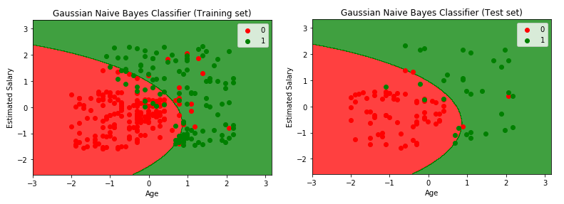
DECISION TREE CLASSIFICATION
Earlier, in the REGRESSION section, we have discussed about Decision Tree Algorithms in detail and observed how Decision Tree Regression algorithm works. In this section, let’s try to understand how the Decision Tree Classification algorithm works. As explained previously, a decision tree is used to predict a target value by learning decision rules from the features after asking a series of questions to the data.
Let us consider the below plot of data consisting of two classes/ categories represented by circle and plus sign respectively.
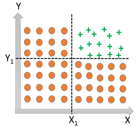
Here, it will not be possible to define a single decision boundary line separating the two classes and we need more than one lines (like in the diagram above) to divide the classes – one separating according to the threshold value of X (X1) and another separating according to the threshold value of Y (Y1).
The Decision Tree Classifier algorithm keeps on dividing the plot into subparts by identifying lines continuously until some criteria of the classifier attributes are fulfilled or it has successfully divided the classes which contain members of a single class.
Entropy and Information Gain
“Entropy” and “Information Gain” are two most important parameters in a Decision Tree Classification problem. Entropy is the degree of randomness of the data and is given by the formula:
Entropy (H) = – ∑ (p(x)*logp(x))
The parameter Information Gain on the other hand helps us to select the best feature for dividing the current working dataset. It tells us how important a given attribute of the feature vector is. If we divide the working set into multiple branches, then the Information Gain at any node is given by the formula:
Information Gain (n) = Entropy (H) – ([Weighted Average]*Entropy(children for feature))
Dividing the working set based on the maximum Information Gain is the key to the success of a Decision Tree Classification Algorithm.
Let us now go through the Python implementation of Decision Tree Classifier using the Car_Purchase dataset.
# Decision Tree Classification

# Import the required libraries and the collected Dataset
import numpy as np
import matplotlib.pyplot as plotter
import pandas as pd
collectedDataset = pd.read_csv('Car_Purchase.csv')
X = collectedDataset.iloc[:, [2, 3]].values
Y = collectedDataset.iloc[:, 4].values

# Split the dataset into the Training set and Test set
from sklearn.model_selection import train_test_split
X_train, X_test, Y_train, Y_test = train_test_split(X, Y, test_size = 0.25, random_state = 0)

# Feature Scale
from sklearn.preprocessing import StandardScaler
standardScaler = StandardScaler()
X_train = standardScaler.fit_transform(X_train)
X_test = standardScaler.transform(X_test)

# Fit the Decision Tree Model to the Training set
from sklearn.tree import DecisionTreeClassifier
decisionTreeClassifier=DecisionTreeClassifier(criterion='entropy',random_state=0)
decisionTreeClassifier.fit(X_train,Y_train)

# Predict the Test set results
Y_predict = decisionTreeClassifier.predict(X_test)

# Make the Confusion Matrix
from sklearn.metrics import confusion_matrix
cm = confusion_matrix(Y_test, Y_predict)

 # Visualize the Training set results
from matplotlib.colors import ListedColormap
X_set, Y_set = X_train, Y_train
X1, X2 = np.meshgrid(np.arange(start = X_set[:, 0].min() - 1, stop = X_set[:, 0].max() + 1, step = 0.01),
                     np.arange(start = X_set[:, 1].min() - 1, stop = X_set[:, 1].max() + 1, step = 0.01))
plotter.contourf(X1, X2, decisionTreeClassifier.predict(np.array([X1.ravel(), X2.ravel()]).T).reshape(X1.shape),
             alpha = 0.75, cmap = ListedColormap(('red', 'green')))
plotter.xlim(X1.min(), X1.max())
plotter.ylim(X2.min(), X2.max())
for i, j in enumerate(np.unique(Y_set)):
    plotter.scatter(X_set[Y_set == j, 0], X_set[Y_set == j, 1],
                c = ListedColormap(('red', 'green'))(i), label = j)
plotter.title('Decision Tree Classification (Training set)')
plotter.xlabel('Age')
plotter.ylabel('Estimated Salary')
plotter.legend()
plotter.show()

# Visualize the Test set results
from matplotlib.colors import ListedColormap
X_set, Y_set = X_test, Y_test
X1, X2 = np.meshgrid(np.arange(start = X_set[:, 0].min() - 1, stop = X_set[:, 0].max() + 1, step = 0.01),
                     np.arange(start = X_set[:, 1].min() - 1, stop = X_set[:, 1].max() + 1, step = 0.01))
plotter.contourf(X1, X2, decisionTreeClassifier.predict(np.array([X1.ravel(), X2.ravel()]).T).reshape(X1.shape),
             alpha = 0.75, cmap = ListedColormap(('red', 'green')))
plotter.xlim(X1.min(), X1.max())
plotter.ylim(X2.min(), X2.max())
for i, j in enumerate(np.unique(Y_set)):
    plotter.scatter(X_set[Y_set == j, 0], X_set[Y_set == j, 1],
                c = ListedColormap(('red', 'green'))(i), label = j)
plotter.title('Decision Tree Classification (Test set)')
plotter.xlabel('Age')
plotter.ylabel('Estimated Salary')
plotter.legend()
plotter.show()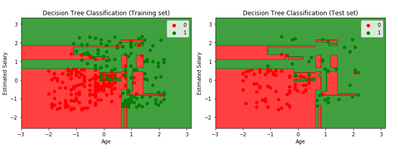
RANDOM FOREST CLASSIFICATION
Like the Decision Tree algorithm, we also discussed about Random Forest algorithm in the REGRESSION section and observed how Random Forest Regression algorithm works.
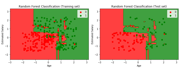
In this section, let’s now try to understand how the Random Forest Classification algorithm works. Random Forest Classification is a Supervised Machine Learning Classification technique which is formed by using the “Ensembling Method” with multiple base Decision Tree Classification models. A high number of Decision Trees in the forest usually gives results with higher accuracy.
Suppose the training set is given as [A1,A2,A3,A4,A5] with labels [L1,L2,L3,L4,L5], then the Random Forest may form 4 decision trees like:
[A1,A2,A4], [A2,A3,A4], [A1,A2,A3], [A1,A3,A4]
From this, it predicts the category based on the plurality vote from the Decision Trees. A single tree might give some noise but by taking into consideration multiple decision tress in a random forest, the effect of noise becomes less which results in a more accurate output.
Random Forest Classification Steps
Step1: Select, at random, “k” number of data points from the training set
Step2: Build the Decision Tree model associated with these “k” data points
Step3: Choose the number of tress (N) you want to build
Step4: Repeat Step1 and Step2
Step5: For a new data point, make each one of your N tree predict the category to which the data points belong and assign the new data point to the category that wins the plurality vote.
Below is the Python implementation of Random Forest Classifier using the Car_Purchase dataset:
#Random Forest Classification

# Import the required libraries and the collected Dataset
import numpy as np
import matplotlib.pyplot as plotter
import pandas as pd
collectedDataset = pd.read_csv('Car_Purchase.csv')
X = collectedDataset.iloc[:, [2, 3]].values
Y = collectedDataset.iloc[:, 4].values

# Split the dataset into the Training set and Test set
from sklearn.model_selection import train_test_split
X_train, X_test, Y_train, Y_test = train_test_split(X, Y, test_size = 0.25, random_state = 0)

# Feature Scale
from sklearn.preprocessing import StandardScaler
standardScaler = StandardScaler()
X_train = standardScaler.fit_transform(X_train)
X_test = standardScaler.transform(X_test)

# Fit the Random Forest Classification model to the Training set
from sklearn.ensemble import RandomForestClassifier
randomForestClassifier=RandomForestClassifier(n_estimators=40,criterion='entropy',random_state=0)
randomForestClassifier.fit(X_train,Y_train)

# Predict the Test set results
Y_predict = randomForestClassifier.predict(X_test)

# Make the Confusion Matrix
from sklearn.metrics import confusion_matrix
cm = confusion_matrix(Y_test, Y_predict)

# Visualize the Training set results
from matplotlib.colors import ListedColormap
X_set, Y_set = X_train, Y_train
X1, X2 = np.meshgrid(np.arange(start = X_set[:, 0].min() - 1, stop = X_set[:, 0].max() + 1, step = 0.01),
                     np.arange(start = X_set[:, 1].min() - 1, stop = X_set[:, 1].max() + 1, step = 0.01))
plotter.contourf(X1, X2, randomForestClassifier.predict(np.array([X1.ravel(), X2.ravel()]).T).reshape(X1.shape),
             alpha = 0.75, cmap = ListedColormap(('red', 'green')))
plotter.xlim(X1.min(), X1.max())
plotter.ylim(X2.min(), X2.max())
for i, j in enumerate(np.unique(Y_set)):
    plotter.scatter(X_set[Y_set == j, 0], X_set[Y_set == j, 1],
                c = ListedColormap(('red', 'green'))(i), label = j)
plotter.title('Random Forest Classification (Training set)')
plotter.xlabel('Age')
plotter.ylabel('Estimated Salary')
plotter.legend()
plotter.show()

# Visualize the Test set results
from matplotlib.colors import ListedColormap
X_set, Y_set = X_test, Y_test
X1, X2 = np.meshgrid(np.arange(start = X_set[:, 0].min() - 1, stop = X_set[:, 0].max() + 1, step = 0.01),
                     np.arange(start = X_set[:, 1].min() - 1, stop = X_set[:, 1].max() + 1, step = 0.01))
plotter.contourf(X1, X2, randomForestClassifier.predict(np.array([X1.ravel(), X2.ravel()]).T).reshape(X1.shape),
             alpha = 0.75, cmap = ListedColormap(('red', 'green')))
plotter.xlim(X1.min(), X1.max())
plotter.ylim(X2.min(), X2.max())
for i, j in enumerate(np.unique(Y_set)):
    plotter.scatter(X_set[Y_set == j, 0], X_set[Y_set == j, 1],
                c = ListedColormap(('red', 'green'))(i), label = j)
plotter.title('Random Forest Classification (Test set)')
plotter.xlabel('Age')
plotter.ylabel('Estimated Salary')
plotter.legend()
plotter.show()